

Marketers today have more control over their advertising investment than ever before. By control, I mean marketers have many options for how to spend their ad dollars, very little commitment in terms of minimum spend levels, and rich data to pour through to measure results. Marketers can reallocate their ad budget weekly, daily, even hourly for certain channels. Despite this flexibility, however, many marketers still use antiquated methods to optimize their ad budgets. Here are six tips to help you systematically boost your marketing performance.
Optimize Lifetime Revenue, Not Sales
Advertising spend is an investment companies can make, similar to investing in new infrastructure, product development, or other worthwhile ventures. There’s an up-front expense for a future payoff. Unlike many other investments, the challenge for marketers is that it can often be difficult to measure the long-term payoff due to lag effects, attribution challenges, and repeat revenue after the point of sale.
Even optimizing based on the cost per sale is not optimal because not all sales are equal.
To simplify things, marketers tend to use lead measures as a gauge for future performance. Metrics like awareness, consideration, response rates, conversion rates, cost per lead, cost per click, click to sale, and cost per call are some of the top-of-funnel and mid-funnel lead measures used in place of actual revenue generation. The problem is, not all clicks, leads, or points of awareness carry the same value. Even optimizing based on the cost per sale is not optimal because not all sales are equal.
For example, certain customers will become repeat customers, leading to repeat revenue over time. Certain customers will purchase more profitable products, be willing to spend more for the same product (lower price elasticity), or purchase higher value products than others. Certain customers will create a lower drain on your operating expense than others (e.g. autopay, paperless billing, online account management). Determining which customers will retain at higher rates, spend more money, or incur lower expenses are all very predictable outcomes that marketers should be using to manage campaigns.
The simplest way to start is by developing a lifetime revenue model on past and present customers, then score sales over the past several months with this lifetime revenue expectation. Aggregate results by marketing channel as you normally would, and observe the lifetime revenue coming from each channel.
As an example, here’s an advertiser that sells a subscription-based product. The chart illustrates lifetime revenue per customer by marketing channel. You can see the difference in average lifetime revenue was nearly 2:1 from top to bottom.
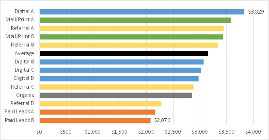
In this case the variability in lifetime revenue is explained by differences in average monthly subscription rates and renewal rates by channel.
For each channel, calculate ad spend as a percent of total revenue generation (cost per sale / lifetime revenue per sale). Then target those channels producing sales at the lowest marketing cost as a percentage of lifetime revenue.
There are several ways you can develop lifetime revenue projections. For subscription-based products, my preference is to separate the exercise into two models: one logistic-based survival model predicting how many months the customer will stay with the company (typically by iterating a logistic model through a geometric series far enough out in time to account for the typical retention tail in that industry), and the second model being a log transformed linear model (log transform your response variable), predicting the revenue each customer provides per month. Then multiply the two predictions together to derive a lifetime revenue projection. This is a common technique in insurance and banking, but it’s equally applicable for any subscription-based service such as mobile phone plans, club memberships and cable/satellite plans.
One challenge analysts face is that typical survival models need a long history of data to make accurate predictions.
Predicting survival rates is the trickier part of this exercise. One challenge analysts face is that typical survival models need a long history of data to make accurate predictions. The weakness of most survival modeling techniques is that your longest-retaining customers tend to have been acquired through different techniques than you’re using today, and typically have a distinct profile from your newer customers. For example, many direct marketers relied much more heavily on direct mail 10 years ago than they do today. Direct mail responders are a distinct consumer profile, and tend to retain for a longer period of time than customers acquired through digital channels. Developing a model on a biased distribution (not representative of your new customer profile) will lead to biased predictions. In this case, you would over-predict survival rates for your newer acquisition channels because they’re under-sampled in your longer-duration customer profile.
Another limitation for typical survival models is your company may lack the historic data because it hasn’t been in existence for very long.
An alternative technique I’ve used to reduce this bias involves developing a two-stage model, using a geometric series to extrapolate the survival curve. In the first stage, take a snapshot of current active customers at the end of one month, then another snapshot a month later, and a third snapshot another month later. Flag the customers from the first month who are no longer customers in the second month, and did not reinstate in the third month. Your predictions will be artificially low if you don’t account for reinstatements. Since you’re using a dataset of current active customers, customers that have been around for 10 years or two days will be included. Most importantly, the distribution of customers you’re modeling will represent current customers, meaning your current marketing tactics will carry more weight with this approach.
Using a logistic regression model, predict the probability of the customer surviving (retaining) 1 month. Make sure to incorporate a ‘months-active’ attribute reflecting the number of months the consumer has been a customer as one of your predictors. It may seem strange that one of the predictors (‘months-active’) seems related to what you’re predicting, but it’s actually not in this model. In this first-stage model, you’re predicting whether or not a customer will stay for one more month, not how many total months the customer will stick around. It subtle, but an important adjustment to make. For many industries, newer customers lapse at a higher rate than existing customers so the retention curve is non-linear. Including this attribute will help the model extrapolate a better survival curve.
With your one-month survival model complete, you can now iterate 1-month survival probabilities in a geometric series for each month up to your maximum, remembering for each prediction to adjust for the current month they’re in. For example, in your first calculation set your ‘months-active’ value to 1 since you’re predicting if a customer will remain from month 1 to month 2. However, in the second calculation, set your ‘months-active’ value to 2 and recalculate the probability. This is the only value that’s changing for each monthly calculation.
Determining how many months you should calculate probabilities is based on how long consumers retain, on average, in your industry. For example, in property & casualty insurance, customers stay with one company for 3-4 years on average, varying widely based on the customer profile from 15 months to around 60 months based on a customer’s credit score, driving record, home value, payment method and number of lines of business insured (auto, home, life, umbrella, RV, health). In this industry I would select a 10 year max customer lifecycle to accommodate a mean around 3.5 years. Otherwise you would cut off too much of the longer-retaining tail. That means 120 calculations.
After the 120 1-month probabilities are calculated, use a geometric series to sum the total number of months the customer is expected to retain. See the table below for an example. Derive the final predicted number of months each customer is expected to retain by summarizing the ‘survival’ column (e.g. s1 + s2 + s3 + … + s120).
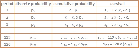
The sum of the ‘survival’ column represents the predicted number of months each customer should retain.
Now for the second stage model. Use a linear regression model to predict the survival months figure you just summarized. Once complete, this final model will provide your survival predictions without needing to compute the geometric series. This method takes more work to develop, but once developed you’ll have a model more applicable to your current marketing tactics.
Lifetime revenue optimization is a little less relevant if you’re selling durable goods such as vehicles, but average revenues still vary by product and inevitably your margins do too.
Even if you’re not ready to transition to a predictive model-based acquisition strategy, this method will at least allow you score historic data and reallocate spend to channels generating greater average lifetime revenue.


Recent Comments