

Optimizing Media Buys in Sportsbook
The rise of Sportsbook
Sportsbook has been rapidly expanding in the United States after the U.S. Supreme Court overturned a federal law that prohibited sports gambling. Originally the Professional and Amateur Sports Protection Act barred state-authorized gambling outside of Nevada. After the May 14, 2018 ruling, states can individually decide to allow sports betting. Currently, 39 states + DC currently allow some form of legalized sports betting and as of April 2026, 30 states allow betting online by mobile app.
In 2025 the industry posted a record revenue of $16.96 billion according to the American Gaming Association. Platforms exist both online (via app) and offline (in-person), with the online market expected to grow at a CAGR of 12.8% from 2025 to 2030.
Sportsbook operators continue to innovate new ways to make sports betting exciting. Special promotions, parlay bets (a single wager combining two or more individual bets), and interactive in-play features during live events are a few. How do you optimize media in a high-growth, highly seasonal industry like Sportsbook?
Media optimization in Sportsbook
OK, so we know it’s a growth industry, which is unique and exciting as a marketer. As each new state legalizes online betting, there’s a mad rush to grab share of wallet as quickly as possible. Pre-launch ads and heavy ad rotation during launch weeks are critical to capture long-term share. Operators know they’re acquiring long-term customers and similar to subscription-based businesses, they’re considering lifetime value in acquisition economics.
Following a new state launch, new activations (customers) stabilize over time and ongoing betting follows the sports calendar (Super Bowl, CFB playoffs, March Madness, NBA finals, etc), meaning less media spend is needed to maintain share. How do you maintain an effective media plan for each new state and each existing state? What should the mix be for new states? Certainly we can learn from the previous state launches, but we’d have to control for time-since-launch and per-capita ad spend due to the vastly different sizes of each market.
But more specifically, how do we ensure the media plan is maximizing lift in sales over what would naturally occur through seasonal demand?
Ultimately we needed a media plan that would optimize spend across four dimensions: time of year, state mix, channel mix, and sub-channel (tactical) allocation.
The setup: data collection for media mix modeling (MMM)
Generally we need: 1) ad spend, 2) sales data, 3) data for sales promotions (special incentives or coupons), and 4) exogenous data that also has an effect on sales volume which is not driven by ad spend – in this case, the sports calendar, estimated consumer interest for each event and competitor data.
We spent several weeks consulting with the client and their vendors to collect ad spend inputs we knew we would need. This included a multi-year dataset of ad spend by media tactic (e.g. TV, programmatic, social, etc), by provider (network, social platform, programmatic vendor, etc), by campaign, by day and by state. This also included campaign-specific details such as bid strategies on social platforms, keyword type (branded, nonbranded, competitor) for search, outdoor ad type for out-of-home ads, and many other breakouts.
Since we were optimizing using expected profit, we needed daily activation volume (new sales) and expected unit profitability based on each market which factored in tax rates and predicted average user betting value by market. We also needed incentive history – A calendar reflecting the dates when incentives were offered and the incentive value (eg Bet $5 and get $300 in Bonus Bets). Finally we compiled search demand for hundreds of sports events over time to help tease out exogenous demand from demand generated through ads.
The approach: an ensemble of machine-learning models
After collecting and normalizing data inputs, we produced multiple modeling datasets with several hundred features, processed through our machine learning framework using an ensemble approach to generate 360 models, each with variations to the training set and slight tweaks in parameters for training set sampling and feature selection methodology (dimension reduction to reduce model overfitting). Non-linear transformations are automatically derived during this process using a Box-Tidwell approach. Some completed models may have as few as 40-50 features used to predict activation volume, or as many as 500 features.
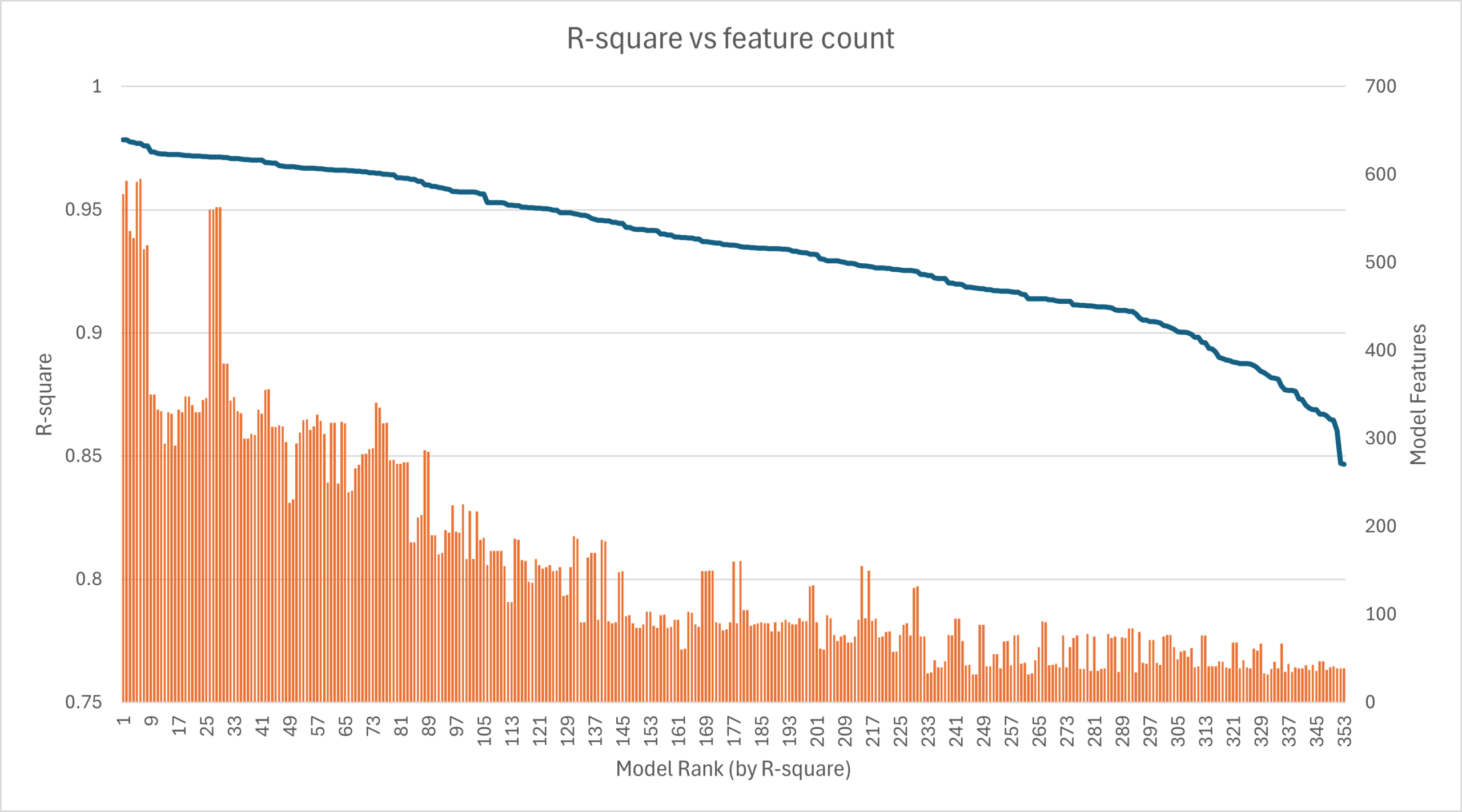
MMM ensemble model ranking by R-square
Typically, models with a high feature count result from less aggressive dimension reduction methods and have the best r-squared fit to the training data but also tend to remain overfit – meaning they fit training data very well but are unstable when validating with simulated data. Models with a low feature count result from more aggressive dimension reduction, and tend to be stable when validating with simulated data but are not reactive enough to variability in training data and essentially underfit the data – leading to the possibility of under-estimating effects within simulated data as well.
The finalist models balance fit and inference. They’re selected based on a combination of fit against training data plus how well they generalize to simulated data (here we’re looking for stability – minimizing extreme predictions).
Simulating the efficient frontier
After modeling we can now simulate hypothetical annual media plans and then predict how many new customers we expect to generate with each media plan. To make sure we were considering a wide range of possibilities, we randomized the ad buys using a monte-carlo process to provide constraints based on a combination of observed historical spend ranges plus some allowed extrapolation to test higher and lower spend levels than what have been observed in the past.
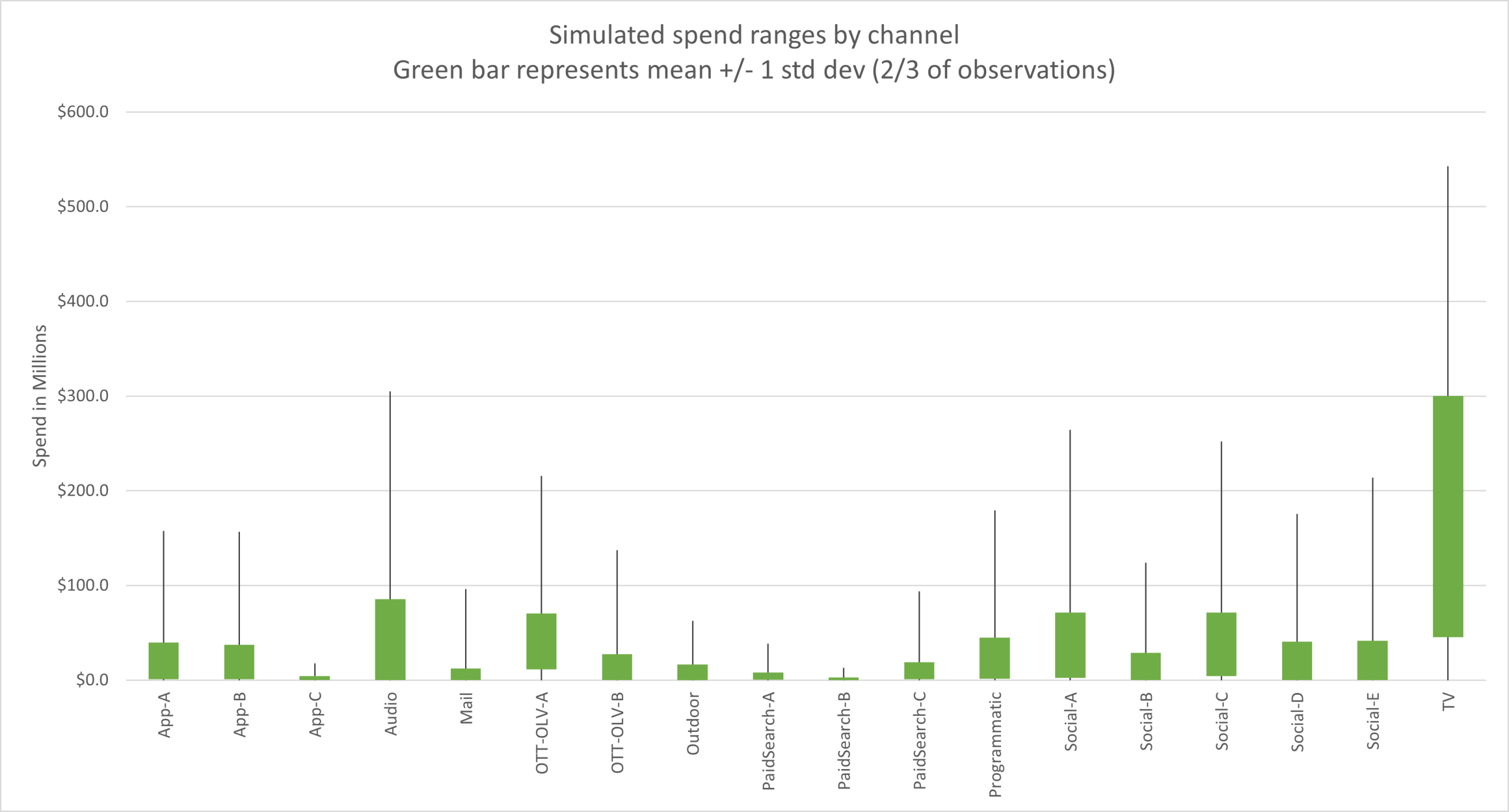
Monte-Carlo spend dispersion by media channel
The optimal ad spend mix is that “efficient frontier” – or leading edge of outcomes for any given spend level. Each dot represents a full annual media plan, with ad spend allocated by state, day, and channel/subchannel.
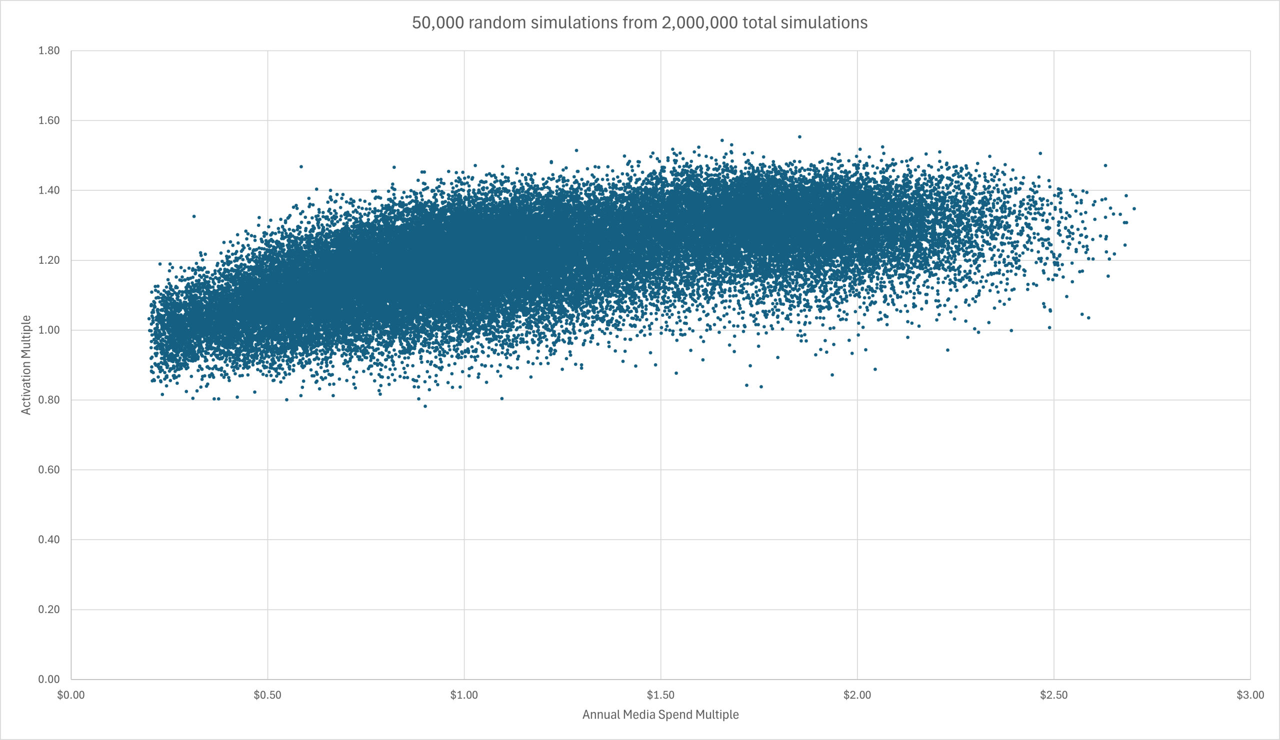
media mix modeling simulation output
Visually we can see that as ad spend (horizonal axis) grows, activation volume (vertical axis) increases at a decreasing rate. That means we have an increasing marginal cost per activation. Both axis have been calibrated to this client’s average spend and activation volume. Media Spend Multiple of $1.0 represents their typical annual budget and Activation Multiple 1.0 represents their observed sales volume. Many simulations offer better results than what this client has been experiencing.
We can estimate baseline sales and the marginal cost per activation using simulated data. Here we can see the exponential marginal cost per activation – meaning ad spend is optimized such that the next new customer should cost more to acquire than the last.
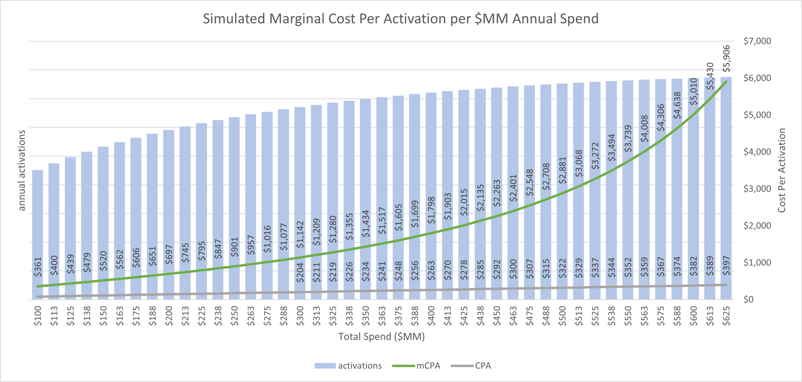
marginal cost per activation
The result: 40% upside?
Media spend reallocations could lead to an increase in new customers by as much as 40%.
That’s a big claim! Admittedly, media mix modeling is identifying correlations, not causations. Which means these findings need to be verified with isolated in-market tests before fully committing the changes. This also implies that spend can be precisely timed throughout the year with no constraints, such as pre-negotiated media spend commitments. But the fact that there is an opportunity to further optimize media spend in such a high-growth industry is good news for everyone.
For this client, changes were needed by media channel, state, and timing throughout the year. In particular, big changes in TV and social mix, reductions in YouTube and audio, quarterly shifts to better align with the sports calendar, and tactical adjustments among several media channels.
The next step is to begin in-market testing to corroborate the findings. Then follow-up with a model recalibration including the latest data reflecting those in-market a/b tests and flighting experiments to confirm if the same mix is still optimal. It’s an ongoing process of identifying opportunities to optimize, leaning into those findings, and confirming results with follow-up measurements.
This process also allows us to estimate baseline sales by quarter, measure incremental new activation volume, estimate marginal cost per activation at varying spend levels, and determine which promotional offers performed the best after controlling for media spend.
For this client, their incremental activation volume dropped substantially in one quarter due to an abrupt drop in media spend where the reductions were not made strategically to cut the poorest performing campaigns. Instead of pulling back surgically, the reductions were more evenly distributed.
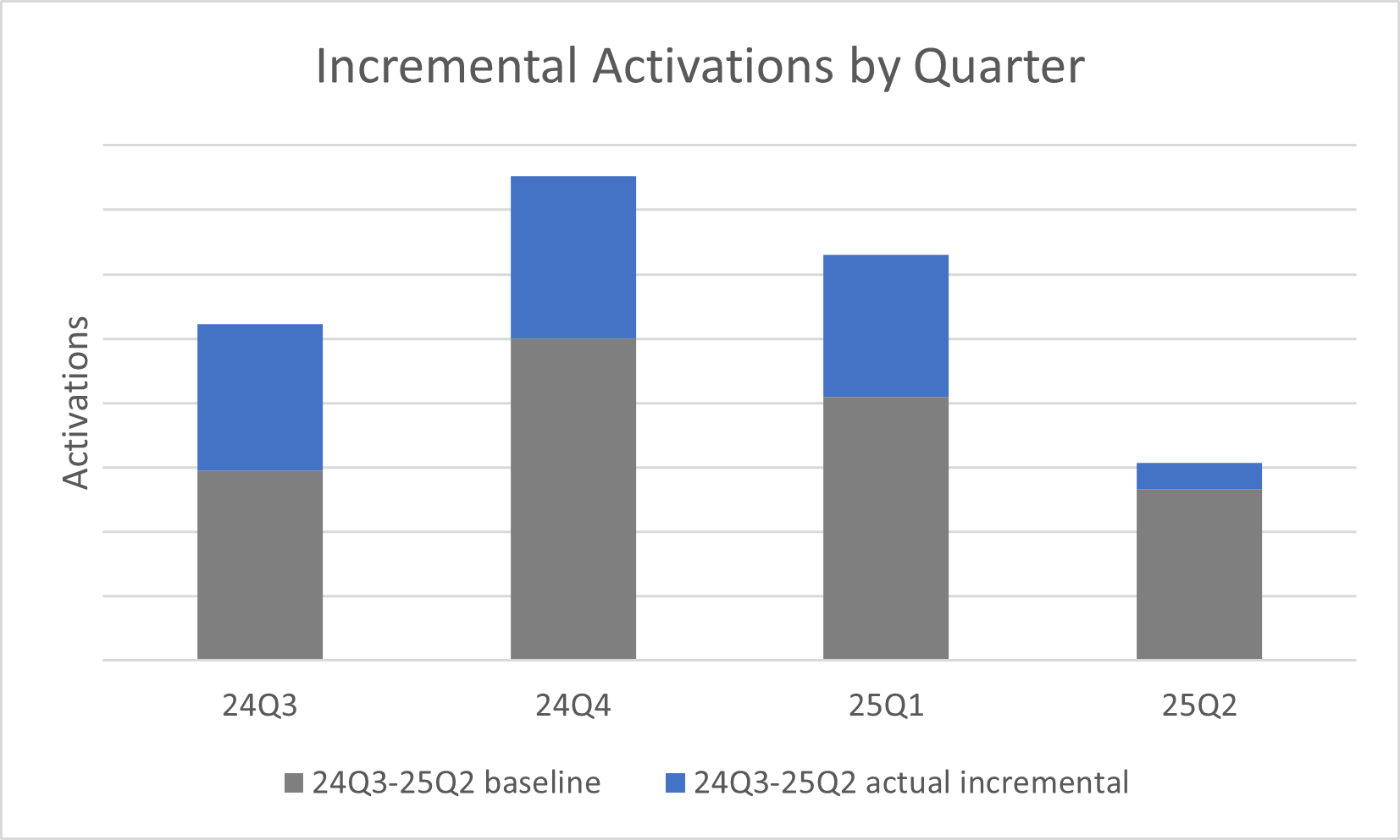
incremental sales over baseline by quarter
Why MineTrove?
There are several vendors offering media measurement, multi-channel attribution, or media mix modeling. Some with more standardized off-the-shelf solutions, some that do not produce simulated forecasts, and many that charge a fortune and then subcontract to firms like MineTrove!
Our approach is bespoke for every client: Custom feature engineering, consultation and advisory support, data QC to ensure the modeling data reconciles with other sources, a proven machine-learning framework to generate highly detailed and precise model predictions, customized monte-carlo simulations to identify the efficient frontier, and strategy consultation to interpret results and make recommendations for next steps. We hope you’ll consider MineTrove on your next MMM project!
NOTE: All exhibits are for illustrative purposes only and all data has been modified from its original version to protect the client.